December | 2012 | Fock Physics

I realize that I need some help with how to proceed to help students discover the principle of momentum in collisions, but before I can adequately explain my problem, I should start at the beginning. I’m trying to refine and improve my technique in building models with students through inquiry so that students can grind their gears on problems that matter and not unimportant details.

The experiments

Before our winter break this year, we started building the Momentum Transfer Model, which, at its start, is really about conservation of momentum. It wasn’t good timing with so little time with which to work. When students watched me collide Cart A (moving) with Cart B (at rest), which would then stick together with Velcro, they suggested various things I could try that might affect the final motion of the carts. They quickly settled on the masses of the two carts and the initial velocity of Cart A. To explore these factors as independent variables, I split students into groups, 1/3 of which were to investigate Cart A’s mass, 1/3 of which were to investigate Cart B’s mass, and 1/3 of which were to investigate Cart A’s initial velocity. As variables go, changing the masses in such a way to keep the total mass constant would be cleaner, but this is hindsight. I wanted to give students a feel for how to gain this kind of hindsight. The groups who experimented with Cart A’s initial velocity had a singularly easy job. They only had to control the variables of the two carts’ masses, and they just pushed Cart A with various speeds and used a motion detector to measure both initial and final velocities. Despite this, some groups didn’t pay attention to whether their data made sense. Some groups had data that showed increasing initial velocities of Cart A but blips where the final velocity of the cars decreased before increasing again. Some groups did notice it, and they rechecked the results until they got something consistent. The groups who experimented with Cart A’s mass also had the second easiest assignment. Despite our shortage of track, they were given an extra piece of track to use as a ramp. Releasing the cart from the same location on the ramp gave their initial velocities an uncertainty of about 2 cm/s. However, even though Cart A’s initial velocity was supposed to be a controlled variable, many students didn’t pay very close attention to it or even try to measure it. Despite this, their data was relatively good. The worst results came from the groups who experimented with Cart B’s mass. Since we lacked enough track to make ramps, we used the spring-loaded plunger on one of the carts to achieve a controlled initial velocity that was uncertain at about the 10% level (maybe 5 cm/s). However, it was easy to have a misfire that would result in a reduced initial velocity. Very few student groups noticed that Cart A’s initial velocity varied wildly in their data. The final tally was that in each of my classes only 1/3 to 1/2 of the data was usable. I would ordinarily send students back to the lab to gather better data. I still may do it, since understanding how to gather data is a more important skill than deriving conservation of momentum from experimental data. However, that’s not what I did.

Reflective interlude on data tables

When students gathered data, I had them fill out all six variables below, not just their independent and dependent variables. This confused them at first but encouraged them to record values and/or measure each of them, which did help them to assess the quality of their data. Unfortunately, when they went to graph it, they were confused about what mattered and didn’t. I probably should have just told them to graph something and then we could argue about whether it was useful later and why. Instead I just grumbled impatiently at students like they were asking me how to breathe. Not super helpful. The, even less helpfully, I gave them what they should graph. Anyway, here’s what they recorded, though I encouraged them to choose the order of the variables that made most sense to them:

A’s mass [cart]	B’s mass [cart]	A’s initial velocity [cm/s]	A’s final velocity [cm/s]	B’s initial velocity [cm/s]	B’s final velocity [cm/s]
				(will be 0 since B’s initially at rest)	(will be the same as A’s final velocity)

Interlude on limiting behaviors

The first day that I realized the data was bad, we just looked at the limiting behavior that we would expect for really small and really large masses. We came up with analogies for each situation, and sketched the graphs. This effectively broke the linear models students fit to their data, but they stared blankly because they hadn’t really gotten that far with their terrible data anyway. Was this useful? I don’t know yet.

What I did

I made simulations…bunches of them:

# Modified version of https://github.com/gcschmit/vpython-physics/blob/master/inelastic%20collision/inelastic.py
### INITIALIZE VPYTHON
# -----------------------------------------------------------------------
from __future__ import division
from visual import *
from physutil import *
from visual.graph import *

### Initial conditions:
# -----------------------------------------------------------------------
mA = 1 # cart
mB = 1 # cart
vA = 24 # cm/s
vB = 0 # cm/s

class QuantityField:
    def __init__(self, pos=vector(0,0,0), variable='', delimeter=' = ', unit=''):
        try:
            self.variable = variable
            self.delimeter = delimeter
            self.unit = unit
            self.label = label(pos=pos, text=(variable+delimeter+'?'+unit), box=False)
        except TypeError as err:
            print('Wrong types passed to QuantityField constructor')
            print(err)
            raise err
    def update(self, q):
        try:
            self.label.text = (self.variable+self.delimeter+str(q)+self.unit)
        except TypeError as err:
            print('Wrong type passed to QuantityField update method')
            print(err)
            raise err

### SETUP ELEMENTS FOR GRAPHING, SIMULATION, VISUALIZATION, TIMING
# ------------------------------------------------------------------------

scene = display(title="Inelastic collision", width=600, height=400, background = color.black)
scene.autoscale = False
scene.range = 2.0

# Define scene objects (units are in meters)
objA = sphere(radius = 0.1*pow(mA,1./3), color = color.green)
objB = sphere(radius = 0.1*pow(mB,1./3), color = color.blue)

# Set up motion map for ball 1
motionMapA = MotionMap(objA, 10, # expected end time in seconds
    10, # number of markers to draw
    labelMarkerOrder = False, markerColor = objA.color, markerScale=0.5, markerType="breadcrumbs")

# Set up motion map for ball 2
motionMapB = MotionMap(objB, 10, # expected end time in seconds
    10, # number of markers to draw
    labelMarkerOrder = False, markerColor = objB.color, markerScale=0.5, markerType="breadcrumbs")

# Set timer in top right of screen
timerDisplay = PhysTimer(0, 1) # timer position (units are in meters)

mADisplay = QuantityField(vector(-1, 0.8, 0), variable="A's mass", unit=' cart')
mADisplay.update(mA)
mBDisplay = QuantityField(vector(1, 0.8, 0), variable="B's mass", unit=' cart')
mBDisplay.update(mB)

ivADisplay = QuantityField(vector(-1, 0.6, 0), variable="A's init.vel.", unit=' cm/sec')
ivADisplay.update(round(float(vA),2))
ivBDisplay = QuantityField(vector(1, 0.6, 0), variable="B's init.vel.", unit=' cm/sec')
ivBDisplay.update(round(float(vB),2))

vADisplay = QuantityField(vector(-1, 0.4, 0), variable="A's velocity", unit=' cm/sec')
vBDisplay = QuantityField(vector(1, 0.4, 0), variable="B's velocity", unit=' cm/sec')

### SETUP PARAMETERS AND INITIAL CONDITIONS
# ----------------------------------------------------------------------------------------

# Define parameters

objA.m = mA # mass of ball in kg
objA.pos = vector(-1, 0, 0) # initial position of the ball in(x, y, z) form, units are in meters
objA.v = vector(vA/100, 0, 0) # set the velocity vector

objB.m = mB # mass of ball in kg
objB.pos = vector(1, 0, 0) # initial position of the ball in(x, y, z) form, units are in meters
objB.v = vector(vB/100, 0, 0) # set the velocity vector

# Define time parameters
t = 0 # starting time
dt = 0.01  # time step units are s

def v_from(obj):
    "helper routine to give cm/sec units from the object's velocity"
    return round(obj.v.mag*100, 2)

### CALCULATION LOOP; perform physics updates and drawing
# ------------------------------------------------------------------------------------

while mag(objA.pos) < 2 and mag(objB.pos) < 2 :  # while the balls are within 2 meters of the origin

    # Required to make animation visible / refresh smoothly (keeps program from running faster
    #    than 1000 frames/s)
    rate(1000)

    # Position update
    objA.pos = objA.pos + objA.v * dt
    objB.pos = objB.pos + objB.v * dt

    # check if the balls collided
    if mag(objA.pos - objB.pos) < ((objA.radius + objB.radius) / 2):
        # calculate the total momentum
        totalMomentum = (objA.m * objA.v) + (objB.m * objB.v)

        # calculate the velocity of the combined ball
        objA.v = objB.v = totalMomentum / (objA.m + objB.m)

    # Update motion map, timer
    motionMapA.update(t)#, objA.v)
    motionMapB.update(t)#, objB.v)
    timerDisplay.update(t)
    vADisplay.update(v_from(objA))
    vBDisplay.update(v_from(objB))
    # Time update
    t = t + dt

### OUTPUT
# --------------------------------------------------------------------------------------

# Print the final time and the ball's final position
#print(', '.join(map(str,["A's mass", "A's initial velocity", "B's mass", "B's initial velocity", "Final mass together", "Final velocity together"])))
#print(', '.join(map(str,[mA, vA, mB, vB, mA+mB, v_from(objA)])))

#print(','.join(map(str,["A's mass", "A's initial velocity", "A's final velocity", "B's mass", "B's initial velocity", "B's final velocity"])))
#print(','.join(map(str,[mA, vA, v_from(objA), mB, vB, v_from(objB)])))

print(','.join(map(str,["A's mass", "B's mass", "A's initial velocity", "A's final velocity", "B's initial velocity", "B's final velocity"])))
print(','.join(map(str,[mA, mB, vA, v_from(objA), vB, v_from(objB)])))

I also threw together a spreadsheet that would automatically calculate the final velocities given the two masses and Cart A’s initial velocity. Then, we played the Hypothesis Game to get students used to finding patterns. Some of mine were too hard, and some were too easy. I need to keep track of those, but that’s a project for another day. Once they had some success finding patterns, we turned to a class speed-round of the Hypothesis Game (but really more like people just sharing their observations&emdash;more cooperation than competition). We took turns by having each group suggest some data to try. This was much cleaner than student data but not as much fun. We came up with data like this (leaving off the two least useful variables, Cart B’s initial and final velocities):

Not very useful for finding patterns
A’s mass [cart]	B’s mass [cart]	A’s initial velocity [cm/s]	A’s final velocity [cm/s]
75	1	25	24.7
100	27932	1000	3.6
5	2	20	14.3
1	2	3	1.0
20	6	11	8.5
7	9	20	8.8

Hmmm, these kids would play Mastermind by choosing random permutations. I suggested something with equal masses and asked what they noticed. We made a connection to the graphs for those who plotted Cart A’s final velocity versus Cart A’s initial velocity and came up with a slope of about 1/2. I asked what would happen if I doubled the masses. They guessed, and we tried it. Then I told them to pick a combination of masses with a total mass of 5. It looked like this (sorted):

Semi-useful for finding a formula
A’s mass [cart]	B’s mass [cart]	A’s initial velocity [cm/s]	A’s final velocity [cm/s]
0	5	60	0
1	4	60	12
2	3	60	24
3	2	60	36
4	1	60	48
5	0	60	60

The equal mass cases that I suggested were enough to get students to look at the fraction $\dfrac{\vec{\boldsymbol{v}}_{Af}}{\vec{\boldsymbol{v}}_{Ai}}$ , and it wasn’t too long before they realized that this fraction was the same as $\dfrac{m_A}{m_A+m_B}$ , and they made rules that turned out to be 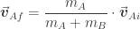$\vec{\boldsymbol{v}}_{Af}=\dfrac{m_A}{m_A+m_B}\cdot\vec{\boldsymbol{v}}_{Ai}$ . We checked it by making predictions and then trying them to see if they were correct. What was nice is that I didn’t have to tell anyone that their formula was wrong. We just tested it.

Here it is, my problem!

Here’s what I don’t get. I can turn the above equation for $\vec{\boldsymbol{v}}_{Af}$ into $m_A\,\vec{\boldsymbol{v}}_{Ai}+m_B\,\vec{\boldsymbol{v}}_{Bi}=m_A\,\vec{\boldsymbol{v}}_{Af}+m_B\,\vec{\boldsymbol{v}}_{Bf}$ by careful mathematical steps. I even tried it with one exceptionally clever class who figured it out a day before my other classes, but I think I might have melted their brains. For kids just out of algebra and now in geometry, manipulating equations with six variables seemed like torture. How do I put the focus on the product of mass and velocity as an interesting conserved quantity? How do I go from the simple equation $\vec{\boldsymbol{v}}_{Af}=\dfrac{m_A}{m_A+m_B}\cdot\vec{\boldsymbol{v}}_{Ai}$ to a deep physical principle?

Update

Based on John’s comment below, I wanted to think about the implicit axioms we use in physics when coming up with formulas.

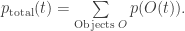
(symmetry) Noether’s Theorem tells us that whenever we find a symmetry of the action, we can write down conserved charges $Q_i=Q_f$ . Total momentum is such a charge, based on the symmetry that the laws of physics are the same at all points in space (i.e. that the action is translation-independent). However, even if we hadn’t identified the symmetry, we have become used to finding conserved (unchanging in time) quantities, so we insist that our conservation equation have the form
$p_i=p_f.$

Doing so ensures that it will be maximally useful: We don’t have to know what’s going on at two different timer readings to calculate our conserved quantity $p$ .
(locality) When we have different objects, we should be able to calculate the conserved quantity one at a time and then combine them somehow. (N.B. Interaction energies might seem to be an exception to this, but once fields are introduced, even energy can be written in a local form.) If we have two objects, $O_A$ and $O_B$ , the functional form of the conserved charge in terms of the properties of the objects shouldn’t depend on what’s going to happen next or on what’s happening very far away. It would be bizarre if we had to calculate it one way if the two objects were going to collide and another way if they weren’t. It would be equally bizarre if we had to calculate it differently depending on whether a star is exploding in another galaxy. Therefore,
$p_{\text{total}}(t)=\sum\limits_{\text{Objects }O}p(O(t)).$

Why does this have to be a sum? The formula has to be well-defined independent of our notion of objects, so considering two different objects to be a single object or a single object to be made of two objects shouldn’t change the answer. There are a limited number of ways of doing this. Actually, one could exponentiate both sides to made it a product instead, or if it’s a product, take the logarithm of both sides to make it a sum.

When dealing with two objects ( $A$ and $B$ ) colliding, we thus want to ensure that our conservation equation has the form

$p(m_A,\vec{v}_{Ai})+p(m_B,\vec{v}_{Bi})=p(m_A,\vec{v}_{AF})+p(m_B,\vec{v}_{Bf}),$

where $p(m,\vec{v})$ is a function of the mass and velocity.

I don’t think that this is the way I’d teach it. It might be enough to leave off the second axiom and just look for a functional form

$p(m_A,\vec{v}_{Ai},m_B,\vec{v}_{Bi})=p(m_A,\vec{v}_{AF},m_B,\vec{v}_{Bf})$

and notice that it has the simple form of the previous equation. When it doesn’t work, what kinds of questions can I ask to focus students on what they are trying?

Post-class update

Something interesting happened while teaching this. My students have one-to-one laptops, which I control strictly. Violate rules on when and how to use them, and you lose all privileges to use laptops until you choose to set up a parent-student-teacher meeting to resolve the issues and decide under what conditions to allow you to use it. This policy has worked well, but that’s a different story. It means, however, that I made a small number of paper copies for those who aren’t currently allowed to use their laptops. I taught the students how to use a spreadsheet to enter a formula and test it to see if their formula using the two mass/velocity pairs was conserved (the same before and after the collision). Presumably, students using paper were partly-ignoring me during this spreadsheet review (difference 1). Entering the spreadsheet formula required four steps (two formulas and two fill-downs), taking up a significant portion of working memory (difference 2). Students working with the spreadsheet tended to focus on different kinds of formulas, whereas students working with the paper copy tended to focus more on the actual numbers and use mental math to see patterns (difference 3). The net result was that of the 5%-10% of my class that found the formula in the 30 minutes I gave them—admittedly low, but I decided to go with the time constraint and have this group explain to the rest—around 2/3 were paper users. I like using spreadsheets, but for a task like this, I think paper wins.

After pointing out that the masses were conserved (individually and together in this case), I did a Think Aloud and looked at the first two rows of data, in which the sum of the velocities was conserved because the object masses were equal. I used this as my idea, which students could immediately see was wrong if they looked at the third data point. This was how I showed them how to enter a formula in the spreadsheet.

Rather than scaffolding with questions, I scaffolded with a series of hints:

Use all four variables $m_A$ , $\vec{\boldsymbol{v}}_{A}$ , $m_B$ , $\vec{\boldsymbol{v}}_{B}$ in the formula.
When adding two quantities, they must have the same units. When multiplying or dividing, it doesn’t matter.
We might expect that since it doesn’t matter which we call “A” or “B”, that the formula will be the same if we switch the “A” and “B” parts.
Since “A” and “B” are separate objects, we might expect the formula to be of the form: (A’s part involving $m$ and $\vec{\boldsymbol{v}}$ )+(B’s part involving $m$ and $\vec{\boldsymbol{v}}$ )

I would reveal a new hint when I saw flagging spirits. I was proud that almost all of the students were trying things. Even when it became clear that I was adding hints, they didn’t stop to wait for better hints but kept at it. I was also super proud of the pair of students who worked out the conserved quantity $\frac{m_A}{m_B}\cdot\vec{\boldsymbol{v}}_{A}+\vec{\boldsymbol{v}}_{B}$ (which violated hints 3 and 4), and we got to discuss which we liked better (being easier to remember, makes more “sense”), 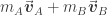$m_A\vec{\boldsymbol{v}}_{A}+m_B\vec{\boldsymbol{v}}_{B}$ or $\frac{m_A}{m_B}\cdot\vec{\boldsymbol{v}}_{A}+\vec{\boldsymbol{v}}_{B}$ , and what was the connection between them. The extension question was: What do you think would be conserved if there were three objects? four? more?

Fock Physics

Building up physics learning one state at a time

Monthly Archives: December 2012

Problem: Marble and tube

Momentum: the little things that trip me up

The experiments

Reflective interlude on data tables

Interlude on limiting behaviors

What I did

Here it is, my problem!

Update

Post-class update

Fock Physics

Building up physics learning one state at a time

Rate this:

The experiments

Reflective interlude on data tables

Interlude on limiting behaviors

What I did

Here it is, my problem!

Update

Post-class update

Rate this: