Lab whiteboarding Defend-the-Model Protocol poster

This is a work in progress, and I encourage feedback. The current version of the poster source code will be at GitHub. Here’s the current PDF (lab-whiteboarding-defend-the-model-beamer-poster-18×24-2013-14-2.pdf) if you don’t have LaTeX.

The idea for the poster comes from Frank Noschese, but blame me for the implementation. As a poster it’s not great yet. The example is just there with no prompts for how to use it. A graph would be helpful. These I’ll add later if the basic idea is sound. It could also do with a different example.

I’ll post images of the various incarnations below.

1st attempt

1st attempt

Update 2013-06-16: Based on feedback from Josh Gates, I’ve changed the last conceptual tool.

2nd attempt

2nd attempt

Rules of Ten: rules of thumb for data collection and processing

Continuing my run making small posters of semi-useful information for physics classes (see Graph Analysis and Mathematical Models), I present the 3rd installment, adapted from Andy Smith’s list that he uses in his class.

rule-of-10-beamer-poster-18×24.pdf

Update: You can now find source code for this and other posters in my GitHub repository.

\documentclass[final]{beamer} % beamer 3.10: do NOT use option hyperref={pdfpagelabels=false} !
%\documentclass[final,hyperref={pdfpagelabels=false}]{beamer} % beamer 3.07: get rid of beamer warnings
\mode<presentation> {  %% check http://www-i6.informatik.rwth-aachen.de/~dreuw/latexbeamerposter.php for examples
\usetheme{default}    %% you should define your own theme e.g. for big headlines using your own logos
\beamertemplatenavigationsymbolsempty
\definecolor{royalblue}{rgb}{0,0.13725490196078433,0.4}
\definecolor{royalblueweb}{rgb}{0.25490196078431371,0.41176470588235292,0.88235294117647056}
\definecolor{burntorange}{rgb}{0.8,0.3333333333333333,0}
\definecolor{silver}{rgb}{0.75294117647058822,0.75294117647058822,0.75294117647058822}
\setbeamercolor{frametitle}{fg=blue!80!black}
\setbeamertemplate{frametitle} {
\begin{center}
\vspace{-2.5cm}\textbf{\insertframetitle} \par
\normalsize\textbf{\insertframesubtitle}
\end{center}
}
\setbeamertemplate{enumerate items}[circle]
\setbeamercolor{structure}{fg=burntorange}
\setbeamercolor{enumerate item projected}{fg=white}
\setbeamerfont{item projected}{size=\normalsize}
\setbeamertemplate{enumerate item}
{
\usebeamerfont*{item projected}%
\usebeamercolor[bg]{item projected}%
\begin{pgfpicture}{-1ex}{0ex}{1ex}{2ex}
\pgfpathcircle{\pgfpoint{0pt}{.75ex}}{1.2ex}
\pgfusepath{fill}
\pgftext[base]{\color{fg}\insertenumlabel}
\end{pgfpicture}%
}

}
\usepackage[english]{babel}
\usepackage[latin1]{inputenc}
\usepackage{amsmath,amsthm, amssymb, latexsym}
\usepackage{bbding}
%\usepackage{times}
%\usefonttheme{professionalfonts}  % times is obsolete
\usefonttheme[onlymath]{serif}
\boldmath
%\usepackage[orientation=portrait,size=a0,scale=1.4,debug]{beamerposter}                       % e.g. for DIN-A0 poster
%\usepackage[orientation=portrait,size=a1,scale=1.4,grid,debug]{beamerposter}                  % e.g. for DIN-A1 poster, with optional grid and debug output
\usepackage[size=custom,width=45.72,height=60.96,scale=1.8,debug]{beamerposter}                     % e.g. for custom size poster (18in x 24in w/ printable 17in x 23in)
%\usepackage[orientation=portrait,size=a0,scale=1.0,printer=rwth-glossy-uv.df]{beamerposter}   % e.g. for DIN-A0 poster with rwth-glossy-uv printer check
% ...
%
\geometry{margin=1in}
\def\imagetop#1{\vtop{\vspace{-1.5cm}\null\hbox{#1}\vspace{-1.5cm}}}
\usepackage{tikz}

\newcommand{\header}[1]{\textcolor{royalblueweb}{\textbf{#1}}}
\newcommand{\spacing}{\vspace{1.0em}}
\newcommand{\parasep}{\vspace{-0.0\baselineskip}\textcolor{silver}{\large\hfill\FiveStar\hfill\FiveStar\hfill\FiveStar\hfill}\vspace{-0.0\baselineskip}}

% From Andrew Smith on MODELING PHYSICS LISTSERVE
\title[Rules of Ten]{Rules of Ten: rules of thumb for data collection and processing}
\author[Vancil]{Brian Vancil}
\institute[Sumner]{Sumner Academy of Arts & Sciences}
\date{2012-04-07}

\begin{document}
\begin{frame}{Rules of Ten}
\framesubtitle{rules of thumb for data collection and processing}
\vspace{-1.5em}\parasep
\begin{enumerate}

\item \header{Collect at least 10 data points.}  A data point is one pairing of independent and dependent variable measurements.  Without enough data points, we cannot reliably find trends in the data. \spacing

\item \header{The largest independent variable measurement should be at least 10 times the smallest independent variable measurement.}  Nature sometimes surprises us at larger or smaller scales than we think to look. \spacing

\item \header{We like the uncertainty in our measurements to be less than 10\% of the range of the measurements.}  There is no point in trying to understand our results mathematically if the variation we see is around the same size as the uncertainty in the measurements. \spacing

\item \header{We like the root mean square error (RMSE) for a fit to be less than 10\% of the range of dependent variable measurements.}  A large RMSE means that our mathematical model does not fit the data very well. \spacing

\item \header{We will consider the vertical intercept negligible if it is less than 5\% of the range of the dependent variable measurements.}  A vertical intercept is likely to be meaningful if it has a decent magnitude compared with our dependent variable measurements.

\end{enumerate}
\spacing\parasep
%\vfill
\begin{center}\footnotesize
Adapted from a list by Andrew~Smith, Air~Academy~High~School, Colorado~Springs,~CO
\end{center}
\end{frame}
\end{document}

Basic Classes of Mathematical Models

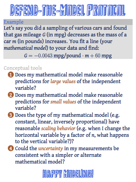
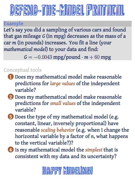
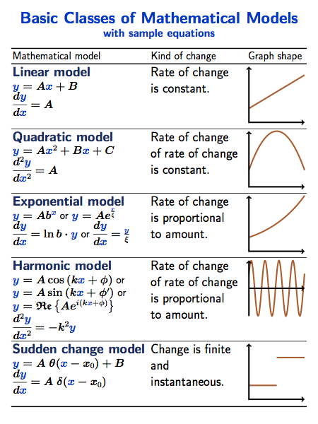
Following David Hestenes on page 6 of Modeling Instruction for STEM Education Reform, I wanted to create a poster like in my previous post of graphical methods and linearizing graphs but this time about the basic classes of mathematical models that Hestenes lists.  I’m not sure that I like all the equation gobbledegook, but I think students need something to which to aspire, so I just made it less prominent.  I’d also like a better presentation of some of the equations.

mathematical-models-B-beamer-poster-18x24
mathematical-models-B-beamer-poster-18×24

Update: You can now find source code for this and other posters in my GitHub repository.

\documentclass[final]{beamer} % beamer 3.10: do NOT use option hyperref={pdfpagelabels=false} !
%\documentclass[final,hyperref={pdfpagelabels=false}]{beamer} % beamer 3.07: get rid of beamer warnings
\mode<presentation> {  %% check http://www-i6.informatik.rwth-aachen.de/~dreuw/latexbeamerposter.php for examples
\usetheme{default}    %% you should define your own theme e.g. for big headlines using your own logos
\beamertemplatenavigationsymbolsempty
\definecolor{royalblue}{rgb}{0,0.13725490196078433,0.4}
\definecolor{royalblueweb}{rgb}{0.25490196078431371,0.41176470588235292,0.88235294117647056}
\definecolor{burntorange}{rgb}{0.8,0.3333333333333333,0}
\setbeamercolor{frametitle}{fg=blue!80!black}
\setbeamertemplate{frametitle} {
\begin{center}
\vspace{-1.2cm}\textbf{\insertframetitle} \par
\normalsize\textbf{\insertframesubtitle}
\end{center}
}
}
\usepackage[english]{babel}
\usepackage[latin1]{inputenc}
\usepackage{amsmath,amsthm, amssymb, latexsym}
%\usepackage{times}\usefonttheme{professionalfonts}  % times is obsolete
\usefonttheme[onlymath]{serif}
\boldmath
%\usepackage[orientation=portrait,size=a0,scale=1.4,debug]{beamerposter}                       % e.g. for DIN-A0 poster
%\usepackage[orientation=portrait,size=a1,scale=1.4,grid,debug]{beamerposter}                  % e.g. for DIN-A1 poster, with optional grid and debug output
\usepackage[size=custom,width=45.72,height=60.96,scale=1.8,debug]{beamerposter}                     % e.g. for custom size poster (18in x 24in w/ printable 17in x 23in)
%\usepackage[orientation=portrait,size=a0,scale=1.0,printer=rwth-glossy-uv.df]{beamerposter}   % e.g. for DIN-A0 poster with rwth-glossy-uv printer check
% ...
%
\geometry{margin=.5in}
\usepackage{array}
\usepackage{booktabs}
\newcolumntype{P}[1]{>{\raggedright\large}p{#1}}
\def\imagetop#1{\vtop{\vspace{-1.5cm}\null\hbox{#1}\vspace{-1.5cm}}}
\usepackage{tikz}

\newcommand{\xx}{\textcolor{variable}{x}}
\newcommand{\yy}{\textcolor{variable}{y}}
\newcommand{\versus}{vs\ }
\newcommand{\plotscale}{2.0}
\newcommand{\plotline}{6pt}
\newcommand{\formatmm}[1]{\textcolor{royalblue}{\textbf{#1}}}
\colorlet{plot}{burntorange}
\colorlet{variable}{blue!80!black}

% From Hestenes' list of 4 basic mathematical models
\title[Mathematical Models]{Basic Classes of Mathematical Models}
\author[Vancil]{Brian Vancil}
\institute[Sumner]{Sumner Academy of Arts & Sciences}
\date{2012-04-07}

\begin{document}
\begin{frame}{Basic Classes of Mathematical Models}
\framesubtitle{with sample equations}
\defaultaddspace=.25em
\vspace{-2cm}
\begin{center}
\begin{tabular}{P{.45\linewidth}P{.29\linewidth}@{\quad}>{\arraybackslash}P{.19\linewidth}} \toprule[.1em]
\normalsize Mathematical model & \normalsize Kind of change & \normalsize Graph shape  \\ \midrule[.1em] \addlinespace

\formatmm{Linear model}
\par \normalsize $\yy=A\xx+B$
\par $\dfrac{d\yy}{d\xx}=A$ &
Rate of change is constant. &
\imagetop{\begin{tikzpicture}[scale=\plotscale,domain=0:4,line width=\plotline,smooth]
\draw[color=plot] plot (\x,.6*\x+1);
\draw[<->] (0,4) -- (0,0) -- (4,0);
\end{tikzpicture}}
\\ \addlinespace \midrule \addlinespace

\formatmm{Quadratic model}
\par \normalsize $\yy=A\xx^{2}+B\xx+C$
\par $\dfrac{d^{2}\yy}{d\xx^{2}}=A$ &
Rate of change of rate of change is constant. &
\imagetop{\begin{tikzpicture}[scale=\plotscale,domain=0:4,line width=\plotline,smooth,samples=40]
\draw[color=plot] plot (\x,{4-0.7*(\x-2)*(\x-2)});
\draw[<->] (0,4) -- (0,0) -- (4,0);
\end{tikzpicture}}
\\ \addlinespace \midrule \addlinespace

\formatmm{Exponential model}
\par \normalsize $\yy=Ab^{\xx}$ or $\yy=Ae^{\frac{\xx}{\xi}}$
\par $\dfrac{d\yy}{d\xx}=\ln b\cdot\yy$ or $\dfrac{d\yy}{d\xx}=\frac{\yy}{\xi}$ &
Rate of change is proportional to amount. &
\imagetop{\begin{tikzpicture}[scale=\plotscale,domain=0:4,line width=\plotline,smooth,samples=40]
\draw[color=plot] plot (\x,{pow(pow(4,.25),\x)});
\draw[<->] (0,4) -- (0,0) -- (4,0);
\end{tikzpicture}}
\\ \addlinespace \midrule \addlinespace

\formatmm{Harmonic model}
\par \normalsize $\yy=A\cos\left(k\xx+\phi\right)$ or $\yy=A\sin\left(k\xx+\phi'\right)$ or $\yy=\mathfrak{Re}\left\{Ae^{i(k\xx+\phi)}\right\}$
\par $\dfrac{d^{2}\yy}{d\xx^{2}}=-k^{2}\yy$ &
Rate of change of rate of change is proportional to amount. &
\imagetop{\begin{tikzpicture}[scale=\plotscale,domain=0:4,line width=\plotline,smooth,samples=40]
\draw[color=plot] plot (\x,{2*cos((\x*6.28-1)r)});
\draw[->] (0,-2) -- (0,2);
\draw[->] (0,0) -- (4,0);
\end{tikzpicture}}
\\ \addlinespace  \midrule \addlinespace

\formatmm{Sudden change model}
\par \normalsize $\yy=A\ \theta(\xx-x_{0})+B$
\par $\dfrac{d\yy}{d\xx}=A\ \delta(\xx-x_{0})$ &
Change is finite and instantaneous. &
\imagetop{\begin{tikzpicture}[scale=\plotscale,domain=0:4,line width=\plotline,smooth,samples=40]
\draw[color=plot, domain=0:2] plot (\x,1);
\draw[color=plot, domain=2:4] plot (\x,3);
\draw[<->] (0,4) -- (0,0) -- (4,0);
\end{tikzpicture}}
\\ \addlinespace

\bottomrule[.1em]
\end{tabular}
\end{center}
\end{frame}
\end{document}